R

R is a language and environment which is a dialect of the S language. R provides excellent facilities for explanatory data analysis via an extensive collection of graphical functions.

Moreover all standard statistical analyses as well as many recent developments are available in built-in packages or in add-on packages. At the moment more than 7700 add-on packages are available.

Go to the home page of the R project to find out more (home page of the R project).

Admittedly R has a steep learning curves and it can be rather time consuming to get to appreciate the way it works. But we would like to encourage everybody keen on doing data analysis to try learning it. It is worth the effort!

Forecaste packages.

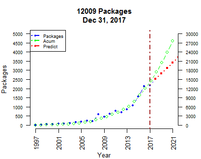
Year	1997	1998	1999	2000	2001	2002	2003	2004	2005	2006	2007	2008	2009	2010	2011	2012	2013	2014	2015	2016	2017
Packages	2	13	57	41	66	66	100	139	187	242	198	572	451	616	777	680	860	1080	1562	2115	2185
AcumPack	2	15	72	113	179	245	345	484	671	913	1111	1683	2134	2750	3527	4207	5067	6147	7709	9824	12009

Forecasts for 5 years. Is it possible?

2018	2019	2020	2021	2022
2526	2824	3122	3419	3717
14535	17359	20481	23900	27617

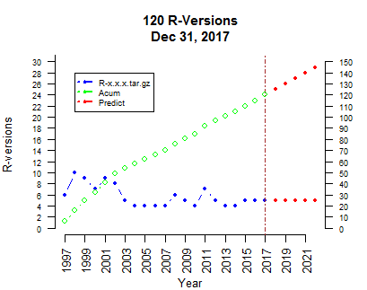
RFreq<-c(6,10,9,7,9,8,5,4,4,4,4,6,5,4,7,5,4,4,5,5,5)
serie <- ts(matrix(RFreq), start=c(1997,1), frequency=1)
fit <- arima( serie, c(0, 1, 1), seasonal = list(order=c(0, 1 ,1), period=1))
# Forecasts for 5 years
P<-predict(fit,n.ahead =5)
Y<-round(c(serie,P$pred),0)
x<-1997:2022
par(mar=c(4,4,4,3),cex=0.8)
plot(x[1:22],Y[1:22],type="b",axes=F,lwd=1.5,ylab="R-versions",xlab="Year",xlim=c(1997,2022),ylim=c(0,30),pch=20,col="blue")
lines(2018:2022,Y[22:26],col="red",type="b",lty=8,lwd=1.5,pch=20)
axis(1,seq(1997,2022,2),las=2)
axis(2,seq(0,35,2),cex.axis=0.7,las=2)
Z<-rep(0,length(Y))
Z[1]<-Y[1]
for(i in 1:(length(Y)-1))Z[i+1]<-Z[i]+Y[i+1]
abline(h=Z[22],v=2017,lty=4,col="brown",lwd=1.5)
par(new=TRUE)
plot(x[1:21],Z[1:21],type="b",axes=F,lwd=1.5,ylab="",xlab="",xlim=c(1997,2022),ylim=c(0,150),col="green")
lines(x[22:26],Z[22:26],col="red",type="b",lty=8,lwd=1.5,pch=20)
axis(4,seq(0,150,10),cex.axis=0.7,las=2)
title(main="120 R-Versions\nDec 31, 2017")
legend(1998,140,c("R-x.x.x.tar.gz","Acum","Predict"),lty=4,col=c("blue","green","red"),cex=0.7,lwd=2,pch=20)
#######

PackFreq<-c(2, 13, 57, 41, 66, 66, 100, 139, 187, 242, 198, 572, 451, 616,777,680,860,1080,1562,2115,2185)
serie <- ts(matrix(PackFreq), start=c(1997,1), frequency=1)
fit <- arima( serie, c(0, 1, 1), seasonal = list(order=c(0, 1 ,1), period=1))
# Forecasts for 5 years
P<-predict(fit,n.ahead =5)
Y<-c(serie,P$pred)
x<-1997:2022
par(mar=c(4,4,4,3),cex=0.8)
plot(x[1:22],Y[1:22],type="b",axes=F,lwd=1.5,ylab="Packages",xlab="Year",xlim=c(1997,2021),ylim=c(0,5000),pch=20,col="blue")
lines(x[22:26],Y[22:26],col="red",type="b",lty=8,lwd=2,pch=20)
axis(1,seq(1997,2022,4),las=2)
axis(2,seq(0,5000,500),cex.axis=0.7,las=2)
Z<-rep(0,length(Y))
Z[1]<-Y[1]
for(i in 1:(length(Y)-1))Z[i+1]<-Z[i]+Y[i+1]
abline(v=2017,lty=4,col="brown",lwd=2)
par(new=TRUE)
plot(x,Z,type="b",axes=F,lwd=1.5,ylab="",xlab="",xlim=c(1997,2022),ylim=c(0,30000),col="green")
axis(4,seq(0,30000,3000),cex.axis=0.7,las=2)
title(main="12009 Packages\nDec 31, 2017")
legend("topleft",c("Packages","Acum","Predict"),lty=4,col=c("blue","green","red"),cex=0.7,lwd=2,pch=20)