Analysis
and comparison between treatment means
The statistical analyses
correspond to the construction of the analysis of variancia and the comparison
of treatments means of the methods established in the library agricolae, as they
are the test of LSD, Tukey, Waller-Duncan, SNK, Duncan and Scheffe. For this demonstration one as far
as possible took the data that are in the library agricolae (version 1.0-9)
Analysis
of the Completely randomized Design and test LSD without formation of
groups To fix the treatments and repetitions (5 treatments with 3
repetition).
library(agricolae)
data(sweetpotato)
model<-aov(yield~virus,data=sweetpotato)
anova(model)
Analysis of Variance Table
Response: yield
Df Sum Sq Mean Sq F value
Pr(>F)
virus 3 1170.21 390.07 17.345
0.0007334 ***
Residuals 8 179.91 22.49
---
Signif. codes: 0 '***' 0.001 '**' 0.01 '*' 0.05 '.' 0.1 ' ' 1
cv.model(model)
[1] 17.16660
mean(yield)
[1] 27.625
comparison <- LSD.test(model,"virus", group=FALSE,
main="Yield of sweetpotato\ndealt with different virus")
Study: Yield of sweetpotato
dealt with different virus
LSD t Test for yield
Mean Square Error: 22.48917
virus, means and individual ( 95 %) CI
yield std.err r LCL
UCL Min. Max.
cc 24.40000 2.084067 3 19.594134 29.20587 21.7 28.5
fc 12.86667 1.246774 3 9.991602 15.74173 10.6 14.9
ff 36.33333 4.233727 3 26.570341 46.09633 28.0 41.8
oo 36.90000 2.482606 3 31.175100 42.62490 32.1 40.4
alpha: 0.05 ; Df Error: 8
Critical Value of t: 2.30600
Comparison between treatments means
Difference pvalue sig
LCL UCL
cc - fc 11.5333333 0.017638 * 2.604368 20.462299
ff - cc 11.9333333 0.015073 * 3.004368 20.862299
oo - cc 12.5000000 0.012088 * 3.571035 21.428965
ff - fc 23.4666667 0.000302 *** 14.537701 32.395632
oo - fc 24.0333333 0.000257 *** 15.104368 32.962299
oo - ff 0.5666667 0.887267 -8.362299
9.495632
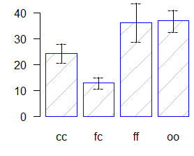
bar.err(comparison$means,variation="std",ylim=c(0,45),density=4, border="blue",las=1)

-
Analysis
of the Design Completely Randomized and test HSD with groups. Previous
case.
comparison <- HSD.test(model,"virus", group=TRUE,
main="Yield of sweetpotato. Dealt with different virus")
Study: Yield of sweetpotato. Dealt with different virus
HSD Test for yield
Mean Square Error: 22.48917
yield std.err r Min. Max.
cc 24.40000 2.084067 3 21.7 28.5
fc 12.86667 1.246774 3 10.6 14.9
ff 36.33333 4.233727 3 28.0 41.8
oo 36.90000 2.482606 3 32.1 40.4
alpha: 0.05 ; Df Error: 8
Critical Value of Studentized Range: 4.52881
Honestly Significant Difference: 12.39967
Means with the same letter are not significantly different.
Groups, Treatments and means
a oo
36.9
ab ff 36.33
bc cc 24.4
c fc
12.87
|
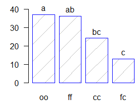
bar.group(comparison$group,ylim=c(0,45),
density=4, border="blue",las=1)
 |
- Comparison
with Waller-Duncan.
It is a Bayesian test, minimizing the two errors: Error I and II.
Appropriate when the researcher is unaware of the behavior of the treatments
and the goal is to make a multiple comparison. This test requires
information from the analysis of variance as the source of the error
variance and the F value calculated with the respective degrees of freedom.
It assigns a value for the test k = 50, 100 or 500, which has some relation
to alpha levels of 0.10, 0.05 and 0.01.
model<-aov(yield~virus,data=sweetpotato)
comparison <- waller.test(model,"virus", group=TRUE, main="Yield of sweetpotato. Dealt with different virus")
Study: Yield of sweetpotato. Dealt with different
virus
Waller-Duncan K-ratio t Test for yield
This test minimizes the Bayes risk under additive
loss and certain other assumptions.
......
K ratio 100.00000
Error Degrees of Freedom 8.00000
Error Mean Square 22.48917
F value 17.34478
Critical Value of Waller 2.23600
virus, means
yield std.err r Min. Max.
cc 24.40000 2.084067 3 21.7 28.5
fc 12.86667 1.246774 3 10.6 14.9
ff 36.33333 4.233727 3 28.0 41.8
oo 36.90000 2.482606 3 32.1 40.4
Minimum Significant Difference 8.657906
Means with the same letter are not significantly different.
Comparison of treatments
Groups, Treatments and means
a oo 36.9
a ff 36.33
b cc 24.4
c fc 12.87.
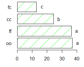
bar.group(comparison$groups,horiz=TRUE,xlim=c(0,45),
density=4,col="green",las=1) |
 |
- Comparison
with Bonferroni, Hochberg, BH, BY and fdr.
(see p.adjust in R).
LSD.test function performs multiple comparisons with adjusted
probabilities. But adjustment is made, the option p.adj = "none", otherwise
it makes adjusting probability.
model<-aov(yield~virus,data=sweetpotato)
LSD.test(model, "virus", p.adj="bonferroni", group=TRUE, main="Yield of
sweetpotato. Dealt with different virus")
Study: Yield of sweetpotato.
Dealt with different virus
LSD t Test for yield
P value adjustment method: bonferroni
Mean Square Error: 22.48917
virus, means and individual ( 95 %) CI
yield std.err r LCL
UCL Min. Max.
cc 24.40000 2.084067 3 19.594134 29.20587 21.7 28.5
fc 12.86667 1.246774 3 9.991602 15.74173 10.6 14.9
ff 36.33333 4.233727 3 26.570341 46.09633 28.0 41.8
oo 36.90000 2.482606 3 31.175100 42.62490 32.1 40.4
alpha: 0.05 ; Df Error: 8
Critical Value of t: 3.478879
Least Significant Difference 13.4704
Means with the same letter are not significantly different.
Groups, Treatments and means
a oo 36.9
a ff 36.33
ab cc 24.4
b fc 12.87
LSD.test(model,"virus", p.adj="bonferroni",group=FALSE, main="Yield of
sweetpotato. Dealt with different virus")
Study: Yield of sweetpotato. Dealt with different virus
LSD t Test for yield
P value adjustment method: bonferroni
Mean Square Error: 22.48917
virus, means and individual ( 95 %) CI
yield std.err r LCL
UCL Min. Max.
cc 24.40000 2.084067 3 19.594134 29.20587 21.7 28.5
fc 12.86667 1.246774 3 9.991602 15.74173 10.6 14.9
ff 36.33333 4.233727 3 26.570341 46.09633 28.0 41.8
oo 36.90000 2.482606 3 31.175100 42.62490 32.1 40.4
alpha: 0.05 ; Df Error: 8
Critical Value of t: 3.478879
Comparison between treatments means
Difference pvalue sig
LCL UCL
cc - fc 11.5333333 0.105827 -1.9370638 25.00373
ff - cc 11.9333333 0.090439 . -1.5370638 25.40373
oo - cc 12.5000000 0.072531 . -0.9703971 25.97040
ff - fc 23.4666667 0.001814 ** 9.9962695 36.93706
oo - fc 24.0333333 0.001545 ** 10.5629362 37.50373
oo - ff 0.5666667 1.000000 -12.9037305 14.03706
- Comparison
with Student-Newman-Keuls SNK.
model<-aov(yield~virus,data=sweetpotato)
comparison <- SNK.test(model,"virus", group=TRUE, main="Yield of sweetpotato. Dealt with different virus")
Study: Yield of
sweetpotato. Dealt with different virus
Student Newman Keuls Test
for yield
Mean Square Error: 22.48917
virus, means
yield std.err r Min. Max.
cc 24.40000 2.084067 3 21.7 28.5
fc 12.86667 1.246774 3 10.6 14.9
ff 36.33333 4.233727 3 28.0 41.8
oo 36.90000 2.482606 3 32.1 40.4
alpha: 0.05 ; Df Error: 8
Critical Range
2 3
4
8.928965 11.064170 12.399670
Means with the same letter are not significantly different.
Groups, Treatments and means
a oo
36.9
a ff
36.33
b cc
24.4
c fc
12.87
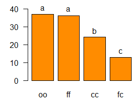
bar.group(comparison$groups,ylim=c(0,45),col=colors()[90],las=1)

- Comparison
with Duncan.
Duncan.test
function performs multiple comparisons with Duncan's new test.
model<-aov(yield~virus,data=sweetpotato)
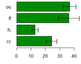
comparison <- duncan.test(model,"virus", group=FALSE, main="Yield of sweetpotato. Dealt with different virus")
Study: Yield of sweetpotato. Dealt
with different virus
Duncan's new multiple range test
for yield
Mean Square Error: 22.48917
virus, means
yield std.err r Min. Max.
cc 24.40000 2.084067 3 21.7 28.5
fc 12.86667 1.246774 3 10.6 14.9
ff 36.33333 4.233727 3 28.0 41.8
oo 36.90000 2.482606 3 32.1 40.4
alpha: 0.05 ; Df Error: 8
Critical Range
2 3
4
8.928965 9.304825 9.514910
Comparison between treatments means
Difference pvalue sig
LCL UCL
cc - fc 11.5333333 0.017638 * 2.604368 20.462299
ff - cc 11.9333333 0.015073 * 3.004368 20.862299
oo - cc 12.5000000 0.014544 * 3.195175 21.804825
ff - fc 23.4666667 0.000388 *** 14.161842 32.771492
oo - fc 24.0333333 0.000387 *** 14.518423 33.548244
oo - ff 0.5666667 0.887267 -8.362299
9.495632
> bar.err(comparison$means,horiz=TRUE, xlim=c(0,45),col=colors()[258],las=1)

- Comparison
with Scheffe.
Scheffe.test function performs multiple comparisons using the Scheffe test,
requires the analysis of variance
model<-aov(yield~virus,data=sweetpotato)
comparison <-
scheffe.test(model,"virus", group=TRUE, main="Yield of sweetpotato. Dealt with different virus")
Study: Yield of sweetpotato. Dealt
with different virus
Scheffe Test for yield
Mean Square Error : 22.48917
virus, means
yield std.err r Min. Max.
cc 24.40000 2.084067 3 21.7 28.5
fc 12.86667 1.246774 3 10.6 14.9
ff 36.33333 4.233727 3 28.0 41.8
oo 36.90000 2.482606 3 32.1 40.4
alpha: 0.05 ; Df Error: 8
Critical Value of F: 4.066181
Minimum Significant Difference: 13.52368
Means with the same letter are not significantly different.
Groups, Treatments and means
a oo
36.9
a ff
36.33
ab cc
24.4
b fc
12.87
